Semantic search works until you add a filter. You search for “wireless earbuds”, get great results, but then you decide to add a filter on brands WHERE brand IN ('Apple', 'Google') and suddenly many results vanish or you get nothing back at all, even if the data has results for your query.

This isn’t a bug in your system but there is a reason why filtering breaks your vector search, and it all has to do with how HNSW works.

This post explains the problem, quantifies how bad it gets, and walks through one of the elegant solutions there exists in vector DBs today which how Qdrant solves it.

1. A quick recap on HNSW

Suppose you’re querying a vector DB with a query embedding q. An easy way to find the nearest neighbors is exhaustive search: compute the similarity between q and all the stored vectors, then take the top k results. That gives exact results but it scales linearly. With N items in your vector DB, you perform O(N) distance evaluations per query. This works great for small datasets but the latency grows rapidly once you start dealing with bigger datasets.

A more realistic way to think about it: imagine you live in a world with no internet and you’re trying to find the best restaurant in an entire country. You wouldn’t inspect every street and every menu. Instead, you’d use a navigation strategy, maybe:

You’ll start by choosing a city that is known for its good restaurants
Then you’ll ask locals and head to likely part of town
Once in there, you’ll ask locals again to go to the right neighborhood
Finally, you’ll only compare restaurants in that neighborhood

At the end of the day, you are trading a tiny risk of missing the absolute best restaurant in the country for a massive speedup.

Approximate Nearest Neighbor (ANN) algorithms formalize this trade-off for vector search. In practice, many vector databases use HNSW (Hierarchical Navigable Small World) as their default ANN index. HNSW builds a graph that lets the query “walk” toward closer and closer candidates without scanning everything.

Btw, if you need a good course about vector search, HNSW and all things related to this, take a look at the free Qdrant Essentials course (not sponsored).

How does it work?

Think back to the “no internet” restaurant problem from the previous section. You want the best restaurant in an entire country. Doing it exactly would mean visiting every street and reading every menu. HNSW turns your “ask the locals” strategy into reality.

The intuition

Your dataset is the country. Each item (vector) is a restaurant somewhere on the map. Your query vector is your personal taste.

HNSW pre-builds “local recommendations”: each restaurant knows a handful of nearby restaurants (nearby in embedding space). At query time, you hop from one promising candidate to the next until you’re in the right neighborhood, then you refine the shortlist.

Under the hood

HNSW stores a graph:

each vector is a node
each node connects to a small set of nearby nodes (neighbors), where nearby is defined by your similarity metric (often cosine)

At query time, the search looks like this:

Start from the index’s entry point (a specific node stored in the HNSW structure).
Keep a shortlist of the best candidates you’ve seen so far.
Repeatedly expand the most promising candidate by checking its neighbors and updating the shortlist.
Stop when your budget is exhausted and return the top $K$ from the shortlist.

The key knob at query time is ef (Qdrant: hnsw_ef) which determines how wide that shortlist is allowed to be. Bigger ef means you consider more alternatives (better recall) but do more distance checks (higher latency).

Here’s a table of the 3 main parameters for HNWS graph and their impact on the usability:

Parameter	When	What it controls	Bigger means…
`M`	build time	max neighbors per node	higher memory, often better connectivity/recall
`ef_construction`	build time	how hard the builder tries to find good edges	slower build, higher index quality
`ef` / `hnsw_ef`	query time	how wide the candidate shortlist is	higher latency, higher recall

Why the hierarchy matters

The strategy above works on a single graph, but it can waste time wandering before it reaches the right region.

HNSW adds the pick the right city first step by using multiple layers for search.

The higher layer is like a very coarse-grained map of the country, including details just about very few restaurant that are very far from each other.
The lowest layer of all is like the map of the whole country with all the details. It includes all the nodes of all previous layer.

In general terms:

upper layers contain fewer nodes with longer-range connections
lower layers contain more nodes with short-range connections

When searching for the most similar nodes to your query, search is top-down.

You start in the top layer, walk greedily to the most similar node you can find until you can’t improve
You drop to the next layer while keeping your current best node as the new starting point
You repeat until the bottom layer (which contains all nodes)

The hierarchy is what makes the navigation both fast and surprisingly accurate.

HNSW greedy search visualization

Source: Qdrant

2. How filtering breaks HNSW

Vector search almost never happens in isolation as your users always want to combine similarity with metadata filters as in our earbuds example: “find wireless earbuds, but only from Apple or Google.”

Two obvious ways to filter come to mind (which are implemented widely in industry) but they both fail most of the time.

The post-filtering method

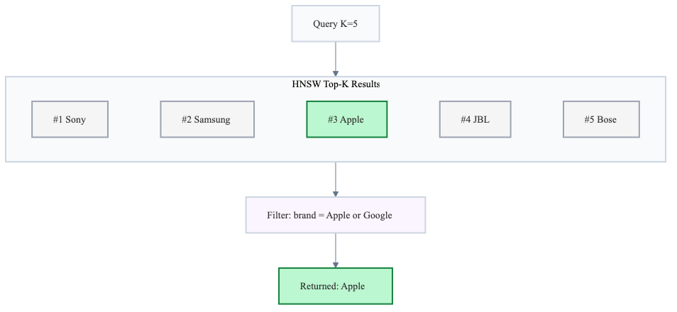
The naive approach: run HNSW to get the top-K most similar results, then throw away the ones that don’t match the filter.

The main reason this method fails is that your top K wireless earbuds results might be dominated by other brands. After discarding non-matching items, you’re left with almost nothing.

HNSW returned 5 results but only 1 matched the filter. Meanwhile, closer Apple/Google earbuds ranked beyond top K were never retrieved, so they could not be returned.

%%{init: {'theme': 'base', 'themeVariables': {'fontFamily': 'Helvetica Neue,Helvetica,Arial,sans-serif', 'fontSize': '14px', 'lineColor': '#64748b', 'textColor': '#0f172a'}}}%%
flowchart TB
  q["Query K=5"]

  subgraph step1["HNSW Top-K Results"]
    r1["#1 Sony"] ~~~ r2["#2 Samsung"] ~~~ r3["#3 Apple"] ~~~ r4["#4 JBL"] ~~~ r5["#5 Bose"]
  end

  f["Filter: brand = Apple or Google"]

  keep["Returned: Apple"]

  q --> step1 --> f --> keep

  style q fill:#f8fafc,stroke:#cbd5e1,stroke-width:2px
  style step1 fill:#f8fafc,stroke:#cbd5e1,stroke-width:2px
  style f fill:#faf5ff,stroke:#cbd5e1,stroke-width:2px
  style r1 fill:#f5f5f5,stroke:#9ca3af,stroke-width:2px
  style r2 fill:#f5f5f5,stroke:#9ca3af,stroke-width:2px
  style r3 fill:#bbf7d0,stroke:#15803d,stroke-width:2px
  style r4 fill:#f5f5f5,stroke:#9ca3af,stroke-width:2px
  style r5 fill:#f5f5f5,stroke:#9ca3af,stroke-width:2px
  style keep fill:#bbf7d0,stroke:#15803d,stroke-width:2px

In practice, you end up making top k higher (and usually the exploration budget ef) high enough that some filtered items make it into the candidate set, which defeats the whole purpose of ANN: you pay for extra work just to throw most of it away.

The pre-filtering method

The other option is to filter the dataset first and then search HNSW only among matching items.

While this method looks sound, it also fails…

The reason it fails is that the HNSW graph was built on all data. When you filter your dataset, you’re removing nodes from the graph, so many edges disappear. Paths between matching items often route through non-matching ones, and once those bridge nodes are gone, the graph falls apart.

%%{init: {'theme': 'base', 'themeVariables': {'fontFamily': 'Helvetica Neue,Helvetica,Arial,sans-serif', 'fontSize': '14px', 'lineColor': '#64748b', 'textColor': '#0f172a'}}}%%
flowchart TB
  subgraph before["Before: Original HNSW graph"]
    direction LR
    apple1["Apple"] --- sony1["Sony"] --- google1["Google"]
  end

  filter["Filter: keep only Apple and Google"]

  subgraph after["After: Sony removed"]
    direction LR
    apple2["Apple"]
    sony2["Sony"]
    google2["Google"]
  end

  before --> filter --> after

  style apple1 fill:#bbf7d0,stroke:#15803d,stroke-width:2px
  style google1 fill:#bfdbfe,stroke:#2563eb,stroke-width:2px
  style sony1 fill:#e9d5ff,stroke:#7c3aed,stroke-width:2px
  style apple2 fill:#bbf7d0,stroke:#15803d,stroke-width:2px
  style google2 fill:#bfdbfe,stroke:#2563eb,stroke-width:2px
  style sony2 fill:#f5f5f5,stroke:#9ca3af,stroke-width:2px
  style filter fill:#f8fafc,stroke:#cbd5e1,stroke-width:2px
  style before fill:#f8fafc,stroke:#cbd5e1,stroke-width:2px
  style after fill:#f8fafc,stroke:#cbd5e1,stroke-width:2px

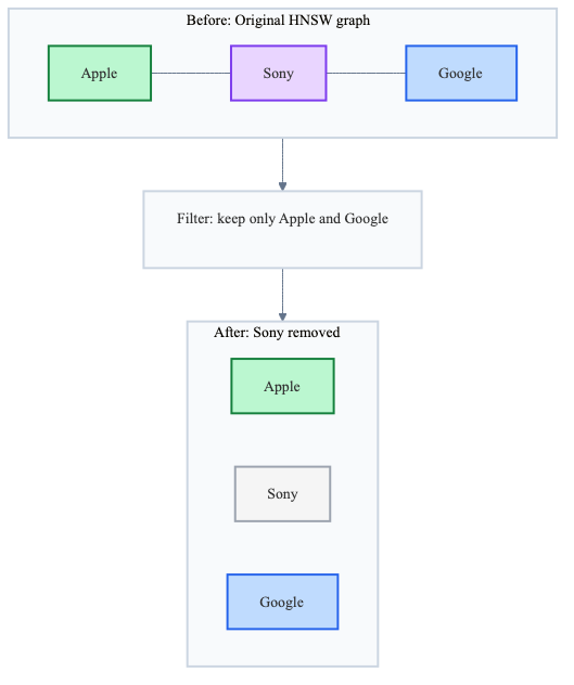
The path from Apple Earbuds to Google Earbuds went through Sony Earbuds. Remove non-matching brands, and Google Earbuds becomes unreachable. Your search silently misses it.

Even worse, if the HNSW entry point (or the early candidates in the queue) happen to be in the filtered-out region, the search may never reach the remaining component at all.

The HNSW graph’s connectivity depends on nodes that your filter removes. This isn’t an edge case — it’s the common case for selective filters.

If you want real numbers on how many nodes you need to keep for a graph to remain connected, I highly recommend reading this short post on HNSW & percolation theory. One caveat: percolation theory assumes random node removal. When filter values correlate with embedding position (e.g., all products of one brand cluster together), removal is spatially correlated — you lose entire neighborhoods at once, which is far more destructive than the random case. The percolation thresholds in that post are optimistic for correlated filters.

3. Qdrant’s solution: filterable HNSW

Not all vector databases/vector frameworks implement a solution for this problem. Many only implement pre-filtering or post-filtering.

Among the providers that do propose a solution, the approaches differ.

In this blog post, I focus on Qdrant’s solution because it is simple and effective.

The idea is to pre-build connected subgraphs for each filter value and merge their edges into the main graph.

How does it work

Filterable HNSW adds a small set of extra edges so filtering does not disconnect matching points.

Take a categorical field like brand with values [Apple, Google, Sony]. Qdrant:

Builds a connected mini-HNSW subgraph inside each brand. That way, the products of each brand become connected together.
Adds those subgraph edges to the main HNSW graph.

This method guarantees that after filtering on brands, points that share the same brand will be connected (reachable from each other).

It’s very important to know that connectivity between different brands is not enforced by these subgraphs. Cross-brand connections rely on similarity links in the main graph, which may or may not survive filtering.

Let us look at an example to make this clear.

In the diagrams below:

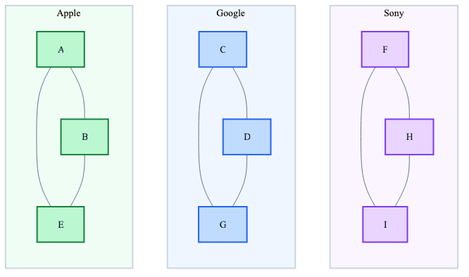
A, B, E are Apple points
C, D, G are Google
F, H, I are Sony

Qdrant builds a graph for each one of the 3 brands.

%%{init: {
  'theme': 'base',
  'themeVariables': {
    'fontFamily': 'Helvetica Neue,Helvetica,Arial,sans-serif',
    'fontSize': '14px',
    'lineColor': '#64748b',
    'textColor': '#0f172a'
  },
  'flowchart': { 'curve': 'basis' }
}}%%
flowchart LR
  subgraph apple["Apple"]
    direction TB
    A["A"] --- B["B"]
    A --- E["E"]
    B --- E
  end

  subgraph google["Google"]
    direction TB
    C["C"] --- D["D"]
    C --- G["G"]
    D --- G
  end

  subgraph sony["Sony"]
    direction TB
    F["F"] --- H["H"]
    F --- I["I"]
    H --- I
  end

  apple ~~~ google ~~~ sony

  classDef appleNode fill:#bbf7d0,stroke:#15803d,stroke-width:2px,color:#0f172a
  classDef googleNode fill:#bfdbfe,stroke:#2563eb,stroke-width:2px,color:#0f172a
  classDef sonyNode fill:#e9d5ff,stroke:#7c3aed,stroke-width:2px,color:#0f172a

  class A,B,E appleNode
  class C,D,G googleNode
  class F,H,I sonyNode

  style apple fill:#f0fdf4,stroke:#cbd5e1,stroke-width:2px
  style google fill:#eff6ff,stroke:#cbd5e1,stroke-width:2px
  style sony fill:#faf5ff,stroke:#cbd5e1,stroke-width:2px

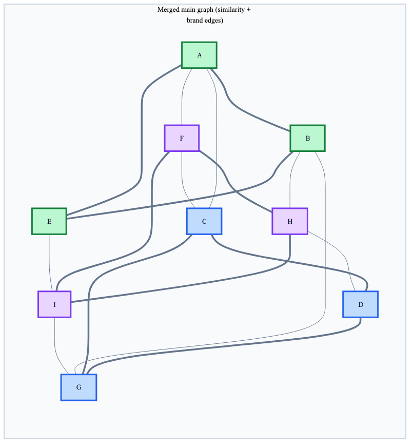
Then these brand graphs are merged into the main graph. This is a key point: after the merge, there’s only one graph in memory containing both:

Similarity edges (from standard HNSW construction which connects nearby vectors using similarity)
Subgraph edges (connecting nodes with the same value of the filter, e.g: brands)

These aren’t stored separately. The subgraph edges are simply added to the existing graph structure at build time.

In the diagram below, all three brands sell similar products (earbuds, headphones, etc.), so their nodes are interleaved in embedding space. That’s why the main graph also has similarity edges across brands including direct Apple <-> Google links.

%%{init: {
  'theme': 'base',
  'themeVariables': {
    'fontFamily': 'Helvetica Neue,Helvetica,Arial,sans-serif',
    'fontSize': '14px',
    'lineColor': '#64748b',
    'textColor': '#0f172a'
  },
  'flowchart': { 'curve': 'basis' }
}}%%
flowchart TB
  subgraph merged["Merged main graph (similarity + brand edges)"]
    direction TB

    subgraph r1[" "]
      direction LR
      A["A"] --- F["F"] --- C["C"]
    end
    subgraph r2[" "]
      direction LR
      B["B"] --- H["H"] --- D["D"]
    end
    subgraph r3[" "]
      direction LR
      E["E"] --- I["I"] --- G["G"]
    end

    %% Cross-brand similarity shortcuts
    A --- C
    B --- G

    %% Brand subgraph edges (thick)
    A === B
    A === E
    B === E

    C === D
    C === G
    D === G

    F === H
    F === I
    H === I
  end

  classDef apple fill:#bbf7d0,stroke:#15803d,stroke-width:3px,color:#0f172a
  classDef google fill:#bfdbfe,stroke:#2563eb,stroke-width:3px,color:#0f172a
  classDef sony fill:#e9d5ff,stroke:#7c3aed,stroke-width:3px,color:#0f172a

  class A,B,E apple
  class C,D,G google
  class F,H,I sony

  style r1 fill:transparent,stroke:transparent
  style r2 fill:transparent,stroke:transparent
  style r3 fill:transparent,stroke:transparent
  style merged fill:#f8fafc,stroke:#cbd5e1,stroke-width:2px

After filtering with brand IN ('Apple', 'Google'), Sony points are removed. Brand subgraph edges keep each brand internally connected. But what about the connection between Apple and Google?

%%{init: {
  'theme': 'base',
  'themeVariables': {
    'fontFamily': 'Helvetica Neue,Helvetica,Arial,sans-serif',
    'fontSize': '14px',
    'lineColor': '#64748b',
    'textColor': '#0f172a'
  },
  'flowchart': { 'curve': 'basis' }
}}%%
flowchart LR
  subgraph filtered["Filtered set (Apple + Google)"]
    direction LR

    subgraph apple["Apple"]
      direction TB
      A["A"] === B["B"]
      A === E["E"]
      B === E
    end

    subgraph google["Google"]
      direction TB
      C["C"] === D["D"]
      C === G["G"]
      D === G
    end

    A --- C
    B --- G
  end

  subgraph removed["Removed (Sony)"]
    direction TB
    F["F"]
    H["H"]
    I["I"]
  end

  classDef appleNode fill:#bbf7d0,stroke:#15803d,stroke-width:3px,color:#0f172a
  classDef googleNode fill:#bfdbfe,stroke:#2563eb,stroke-width:3px,color:#0f172a
  classDef removedNode fill:#f5f5f5,stroke:#9ca3af,stroke-width:2px,stroke-dasharray:6 5,color:#9ca3af

  class A,B,E appleNode
  class C,D,G googleNode
  class F,H,I removedNode

  style filtered fill:#f8fafc,stroke:#cbd5e1,stroke-width:2px
  style apple fill:#f0fdf4,stroke:#cbd5e1,stroke-width:2px
  style google fill:#eff6ff,stroke:#cbd5e1,stroke-width:2px

  style removed fill:#ffffff,stroke:#cbd5e1,stroke-width:2px,stroke-dasharray:6 5

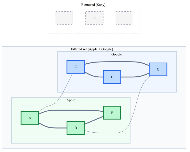
In our example, because Apple and Google sell similar products, their nodes are close in embedding space. The direct Apple <-> Google similarity edges (A–C, B–G) survived the filter, so the search can still jump between brands.

But these cross-brand edges exist because the brands overlap in what they sell. If instead one brand only made luxury laptops and the other only budget wireless earbuds, their products would land in different regions of the embedding space and there would be very few or no similarity edges between them. In that case, after filtering, the search starts in one brand’s cluster and never reaches the other. That’s the pre-filtering failure mode all over again, just at a smaller scale.

Keep this in mind: Filterable HNSW guarantees that all Apple products stay connected and all Google products stay connected. It does not guarantee that Apple products can reach Google products, this really depends on whether similarity edges bridge the gap, which depends on how correlated brand identity is with embedding position.

For single-value filters (e.g., brand = 'Apple'), this distinction doesn’t matter.

Does the memory explode ?

The memory usage is kept well under control with filterable HNSW

As each node belongs to exactly one brand,each node gains at most m additional edges from its brand subgraph, which makes the number of new edges at most n * m. Now, as you add more filters (not only the brand), you’re going to have additional edges built.

The query planner

At query time, Qdrant estimates filter selectivity and decides: should I traverse this graph, or just brute-force?

High or medium selectivity: In this case, Qdrant just traverses the graph. The subgraph edges are always there and whether they’re critical depends on how many nodes the filter removes.
With high selectivity (e.g, 70% match), most similarity edges still lead to valid nodes
With medium selectivity (e.g, 15% match), the subgraph edges become essential for maintaining connectivity.
Low selectivity (e.g, 0.1%): Qdrant skips the graph entirely. When only a tiny fraction of nodes match, brute-force scanning over the filtered set is faster than graph traversal.

The intuition: graph-based search only pays off when there’s enough connectivity to navigate. For very selective filters, there’s so little data left that exhaustive search wins.

Qdrant allows you to control this behavior using full_scan_threshold. When the filtered candidate count falls below full_scan_threshold, Qdrant automatically switches to brute-force scanning.

from qdrant_client.models import VectorParams, Distance, HnswConfigDiff

client.create_collection(
    collection_name="products",
    vectors_config=VectorParams(size=384, distance=Distance.COSINE),
    hnsw_config=HnswConfigDiff(
        m=16,
        ef_construct=100,
        full_scan_threshold=1000  # switch to brute-force when fewer than 1k candidates match
    )
)

Getting it right in practice with Qdrant

Two implementation details trip people up consistently.

1. Create payload indexes explicitly

Qdrant does not automatically index payload fields. Filtering still works without indexes — you’ll get correct results — but you lose two critical optimizations:

No subgraph edges: The HNSW graph won’t have the extra edges needed for filtered search, so you lose the connectivity guarantees described above.
Poor cardinality estimation: The query planner can’t accurately estimate how many points match the filter, leading to suboptimal search strategies. I couldn’t find the exact way it determines the strategy in the documentation but as they’re also an open-source package, the curious minds can dive into their package to get this information.

2. Create indexes before uploading data

The order matters. HNSW graphs only get the subgraph edges when they’re built after the payload index exists. If you upload data first, the HNSW graph gets built without them.

If you already uploaded data without indexes, you can still fix it but you’ll need to force an HNSW rebuild, which is expensive for large collections.

What about numerical filters?

Everything above focused on categorical filters like brand IN ('Apple', 'Google'). But applications also filter on prices, ratings, timestamps, and other continuous values.

Qdrant supports three numerical index types: integer, float & datetime

How Qdrant handles numerical ranges

The original filterable HNSW article explains the approach:

“Numerical range case can be reduced to the previous one if we split numerical range into buckets containing equal amount of points. Next we also connect neighboring buckets to achieve graph connectivity.”

Here’s how the mechanism works:

Buckets contain equal amounts of points . If you have 10,000 products and 10 buckets, each bucket contains ~1,000 products regardless of how prices are distributed.
Neighboring buckets are connected so range queries like products whose price in [150, 350]can traverse across boundaries.
Border filtering is required: items in boundary buckets that don’t match the actual filter need post-filtering. For example, with a price < 150 filter, if bucket boundaries fall at $0, $100, $200, etc., the query would:
- Traverse all buckets up to the one containing $150
- Post-filter items in the boundary bucket to exclude those with price >= $150

This works well in practice but isn’t as clean as the solution for categorical data.

And of course, you can always opt for bucketing the numerical filter data yourself as you might have a better knowledge of the data and of where the boundaries should go.

4. Conclusion

There are really a couple of takeaways here:

Vector search with filters doesn’t just work out of the box and is not just “vector search + WHERE clause
Your Vector DB solution might not provide a solution for this, so do what any sound developer woud do, read the docs !

Why filtering breaks your vector search